My Other Computer is Your Computer - Malware Classification | Akash Trehan

My Other Computer is Your Computer - Malware Classification

May 06, 2018

Malware

Source: https://www.cyberpointllc.com/images/svcs/img-mare.jpg

Background

Why this project?

This project emerged for fulfilling a requirement of the Machine Learning course (EE 769) I took this semester. As I have always been interested in computer security, I wanted to combine my newly learnt knowledge from this course with it. The attacks last year from malwares like WannaCry, NotPetya and Bad Rabbit had made me curious about how these attacks could be prevented. Malware Classification was the perfect project. For this I teamed up with my good friend Mukesh Pareek who is also a security enthusiast. This post is written in collaboration with him. Our guide for this project is Prof. Amit Sethi.

Malware

Malware Classes

Source: http://thepcworks.com/malware/

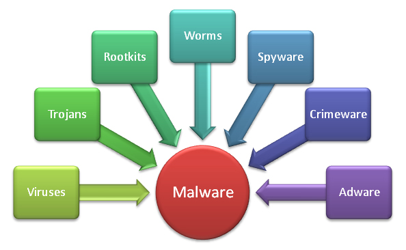
Wikipedia defines malware as:

Malware, short for malicious software, is an umbrella term used to refer to a variety of forms of hostile or intrusive software, including computer viruses, worms, Trojan horses, ransomware, spyware, adware, scareware, and other intentionally harmful programs.

The definition tells us that there are many classes of malware. These categories are made based on how the malware propagates as well as what its intent is.

The Problem

On hearing about malware classification two things come to mind:

Separating malware from benign files
Given a malware, identifying which class the malware belongs to

We focused on solving the second problem.

But why classify malware into classes? Just like a doctor can treat you better if he/she knows what disease you have, anti-malware softwares like antiviruses can defend better if they know the class of malware they are dealing with.

Challenges

Earlier malware was detected using signatures. So whenever there a new malware was found, the companies created its signature and any file whose signature matched was detected. Since this method could only find exact matches, it was very restrictive. Later people shifted to identifying “indicators” which were the defining properties of a class of malware. So if a file had certain indicators it could be classified to the corresponding class. But this again uses only known indicators. With new methods to obfuscate and polymorphism techniques, the creators of these malwares were easily able to get across this layer of protection. The problems we face today is that millions of samples of malware spread everyday. Most of these are duplicates or slight modifications of one another made to decieve the defense systems. Classifying malware thus becomes a daunting task.

Why Machine Learning?

In today’s data rich world, machine learning has become ubiquitous. With its ability to find useful pieces of information from data, machine learning has lead to great results. The defense against a malware attack depends on the broader category of malware and not necessarily on the specific attack sample. This is why machine learning can be used. It can find hidden relationships among the various features of the samples and then leverage those to classify unknown samples.

More specifically…

Now we come to what exactly is the information we have about the malware and what categories do we need to classify it to.

For every malware sample, the input we have is:

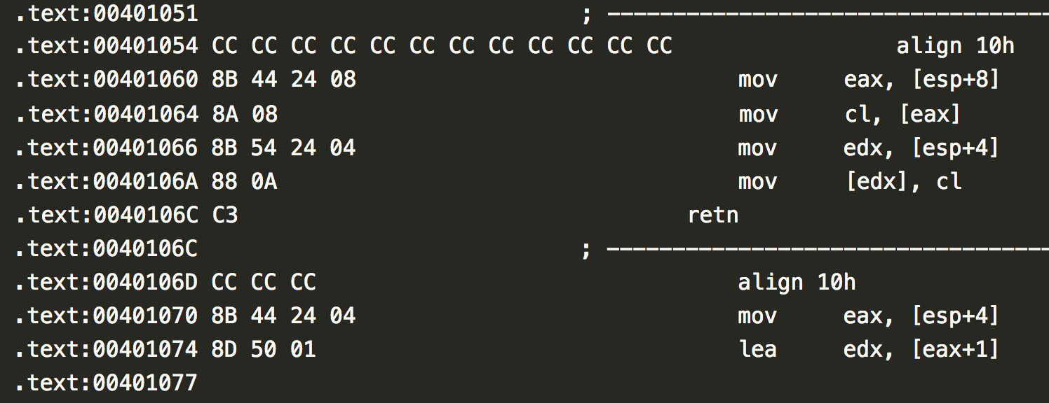
.asm file - This contains the assembly code for the malware program and can be used to extract information about instruction calls, segments etc.

Screenshot of .asm file

Snippet from asm file

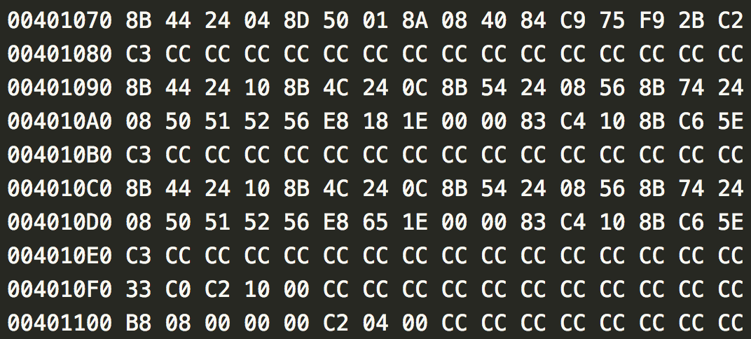
.bytes file - This contains the hexadecimal representation of the file’s binary content. It can be used to extract infomation about the lower level functioning of the malware.

Screenshot of .bytes file

Snippet from bytes file

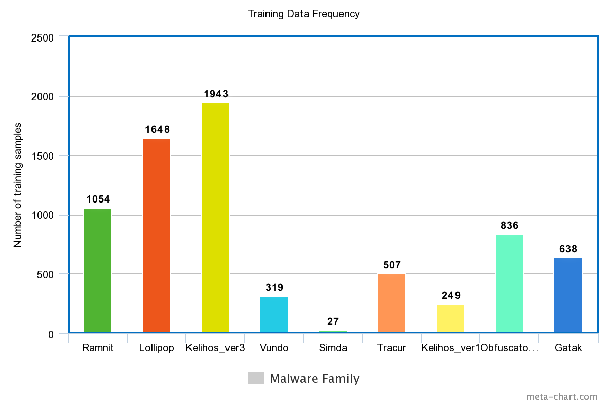
So these two files need to be used to classify the malware into the following 9 families:

Ramnit
Lollipop
Kelihos_ver3
Vundo
Simda
Tracur
Kelihos_ver1
Obfuscator.ACY
Gatak

The dataset

The specific problem as stated above is taken from a malware classification challenge organised by Microsoft on Kaggle. The dataset was also taken from there. The dataset contained 200 GB of training data and 200 GB of test data. Since we didn’t have the labels for the test data, we divided the training data itself into two parts one of which we used for testing purposes. The testing part was half the size of the training part with training having 7221 samples and test having 3648 labels. This divison was done randomly but ensuring that enough members of each class were are a part of both the training and test set.

Each malware sample had a 20 character long ID. We had a csv contatining the ID to Class mapping of the training samples.

Dataset Class Graph

Preprocessing and Feature Extraction ¹

The features we used for classification are as follows:

Instruction n-gram from .asm file - We extracted a list of instructions from the .asm file and used the count for each instruction (1-gram) and instruction-instruction pair (2-gram).
Byte n-gram from .bytes file - We used the hexadecimal representation to extract the byte sequence of the actual malware. Then we used the 1-gram and 2-gram count as our features
Segment Size - We store the number of lines in each of the segments - Header, Data, Text etc. This information is extracted from the .asm files
Pixel Intensity of .asm files - We converted the .asm file into an image and then extracted the last 1000 pixels of the image as features

Our intuition behind using instruction n-grams was that samples from the same class of malware should have similar code and hence there should be similar instructions sequences present in the code. n-grams were a way to represent that. Likewise for the byte n-grams. Using segment size is again based on the intuition that the amount of static data, the amount of space required for the code would be similar for the same class.

Implementation details

Extracting the above features involves text processing and parsing. For this we used the pyparsing python library. The library can be used to specify token formats which make it easier to identify the required instructions or bytes. For getting an image from the .asm file we used byte arrays.

For speeding up the feature extraction we used the ProcessPoolExecutor from concurrent library which made sure that all the cores were being used for processing.

After extracting the features we dumped them to a file so that the processing need not be done again.

Write about feature selection

Training

We used the following models/techniques for learning:

Support Vector Classifier
Xtreme Gradient Booster
Logistic Regression
K Nearest Neighbour Classifier
Random Forest
Neural Network

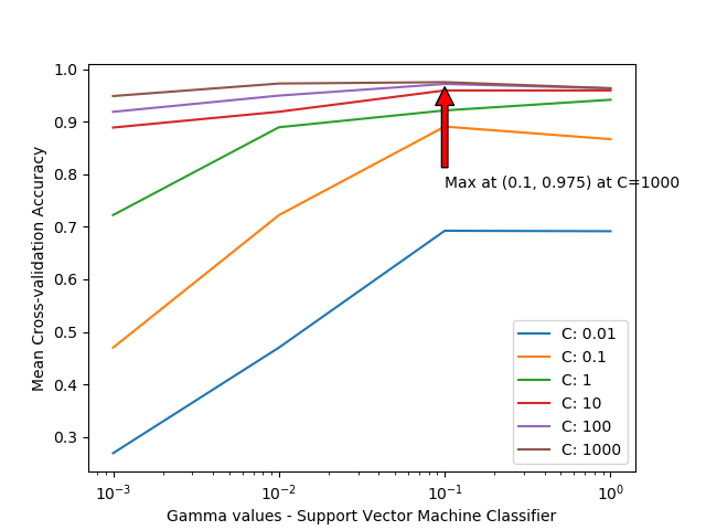
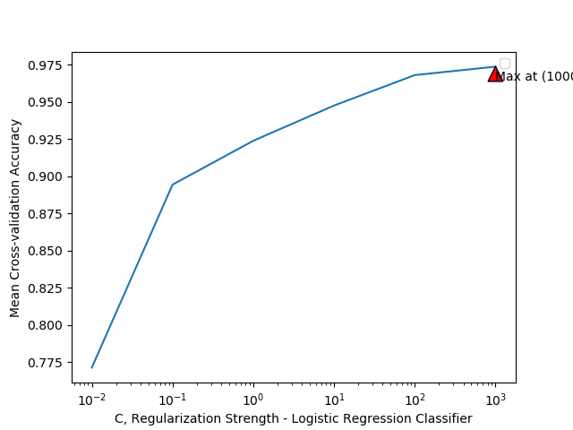
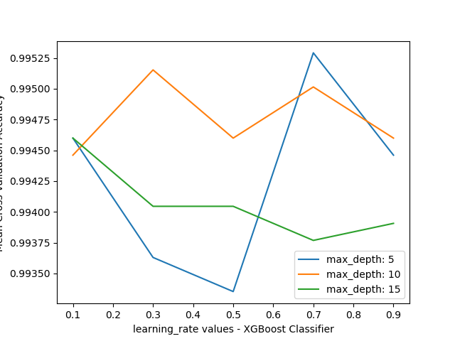
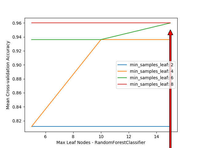
For each of these models we did hyperparameter tuning to find out the best model. Grid search was used to try out all combinations for the values of hyperparameters. We used k-fold cross validation with k=4 for training. To make efficient use of our CPUs we did the grid search in parallel since training of each hyperparameter combination is independent of the other. We used sklearn and xgboost libraries to help us with training.

Evaluation

Hyperparameter Tuning

The graphs for hyperparameter tuning are as follows:

svc

Support Vector Classifier

svc

K Nearest Neighbour Classifier

svc

Logistic Regression

svc

Xtreme Gradient Booster

svc

Random Forest Classifier

Cross Validation and Test Set Accuracy

Model	4-Fold Cross Validation Accuracy	Test Set Accuracy
Logistic Regression	0.9745187647140285	0.910562449264865
Support Vector Classifier	0.9775654341503947	0.869346629
Neural Network	0.941	0.893875612342112
K Nearest Neighbour Classifier	0.9641323916355076	0.821231293817848
XGBoost	0.9945990859991691	0.921231623812763
Random Forest	0.9609472372247612	0.88658497372

We find that we get very good cross-validation accuracies with all models but XGBoost works the best.

XGBoost still dominate all the other models in case of test set but Logistic regression and neural networks also come quite close.

Problems faced and Learning

What did not work is as important as understanding what worked. This section talks about the challenges we faced during this project and what we learned from them. Firstly was the number of features. We wanted to take higher n-grams but the number of combinations were too many leading to very slow training. To get across this hurdle we decided to use Random Forest feature selection so that other models need not train on all the features but only the most important ones.

We were also trying to account for loops in the .asm files while getting the instruction counts. But since we can only do static analysis of the files, we could only follow unconditional jumps which would not have been very useful.

Since we were trying out various techniques we hadn’t used before, we decided to apply semi-supervised learning. But later we learnt that it is used when we have a small amount of labelled data and a large amount of unlabelled data. Then we also use the unlabelled data for learning. Since we didn’t have any shortage of samples, we decided not to do this.

We also wanted to try out Deep Learning but due to the large size of the files (~100 MB for many of the .asm files) it would have been very slow without extracting features manually first to decrease the size.

A major problem we faced was the huge size of the data. We didn’t have enough space on our computers to store all the training data so we had to store it on a server and then run all our code there. After doing this a few times, we came up with the idea that we should just dump the features after extracting them the first time. Then we can read directly from the dumps. This reduced the size from 200 GBs to ~1GB! We thought we were done but then we ran short of another resource - the RAM. All the features from all the data did not fit inside the RAM. A better idea at this point would have been to do batch learning, but we ended up just training on a smaller amount of data due to lack of time.

We learnt a lot about practical ML lessons during the project which increased our understanding significantly.

Conclusion and Future Work

We got good enough accuracy with the data and the low computational resources we had. Thus we can conclude that machine learning can be an effective technique for malware classification. Infact it is extensively being used in industrial applications these days.

Inspite of all the success, machine learning models aren’t full-proof too. The datasets used to train the models are usually biased because there is no common data sink for malware samples. This is caused by the lack of collaboration in the industry.

In future, we would like to try out more models and try more combination of features to find out which ones work best together. We will also make a web front-end for the application where people can upload malware samples and in the backend we use our models to predicts it’s class. This would make this project a complete ready to use package for the users.